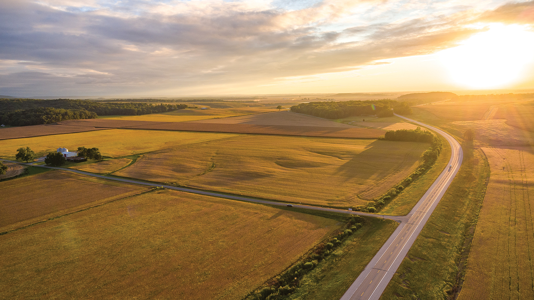
Farmland markets have experienced a remarkable surge in price across much of the country during the last 9 to 12 months with many areas in the Midwest up 20% or more. Farm incomes have been buoyed by strengthening commodity prices, which were supported by increased export demand and recovering domestic usage as well. And all asset market valuations have continued to be supported by sustained low interest rates.

Concern about potential inflation and debate about future monetary policy and stimulus spending regularly generate headlines about future asset values. And unfortunately, disruptions related to the COVID-19 pandemic and associated policy responses have continued longer than expected. In last year’s Market Overview, major issues affecting agricultural asset markets were identified, and it was noted that the demand-side factors supporting continued strong performance would determine near-term performance and that longer-term issues would depend more critically on capital market and interest rate impacts. The reasonably positive projections from a year ago have in fact turned out to be mostly accurate, and the strong market for farmland that developed since then has continued into the fourth quarter which has traditionally been a strong annual season for farmland markets. 

To help provide additional grounding in the performance of agricultural assets as well as the prospects for the future, updated data on national land values, income versus appreciation prospects, and potential impacts of future interest rate and inflation regimes are provided.

FARMLAND MARKETS TODAY HOW DID WE GET HERE?

Agricultural land can be classified by use and type including cropland, pastureland, and a third category that combines all farmland and real estate including buildings and fixtures. Cropland is further divided into the categories of annual row-crop production (e.g., corn, soybeans) and permanent crops (e.g., citrus, tree nuts, wine grapes). USDA publishes the results of its annual survey of land values and lease rates by category along with related information about acreage and use changes, and NCREIF provides complementary information on a quarterly basis on performance of institutionally owned and professionally managed agricultural assets. 

Cropland values are influenced by the type of crop grown and relative productivity, and generally reflect the income earning potential of the agricultural production in that location.

Figure 1 shows 2021 average cropland values by state, and Figure 2 shows the percentage change in value from one year ago. Since the release of the updated USDA data, regional surveys in the Midwest in particular have shown an even more rapid increase in the second half of 2021. Moreover, the USDA data are for all cropland including small and hobby holdings, not solely that which would be considered commercially viable. As a result, USDA data are often viewed as understating prices and financial performance relative to farmland that farmers and investors consider to be investment grade primarily for agricultural production value.

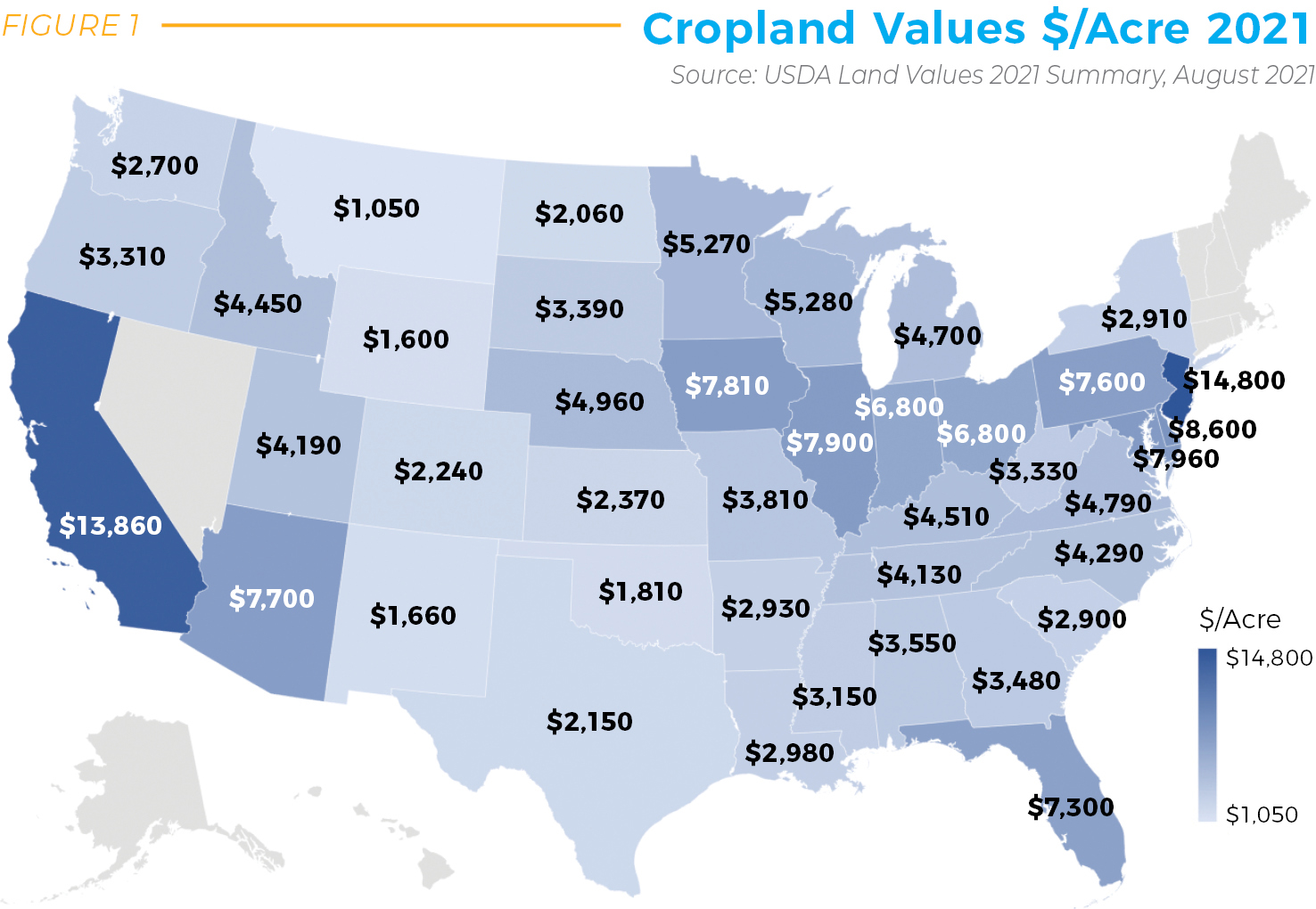
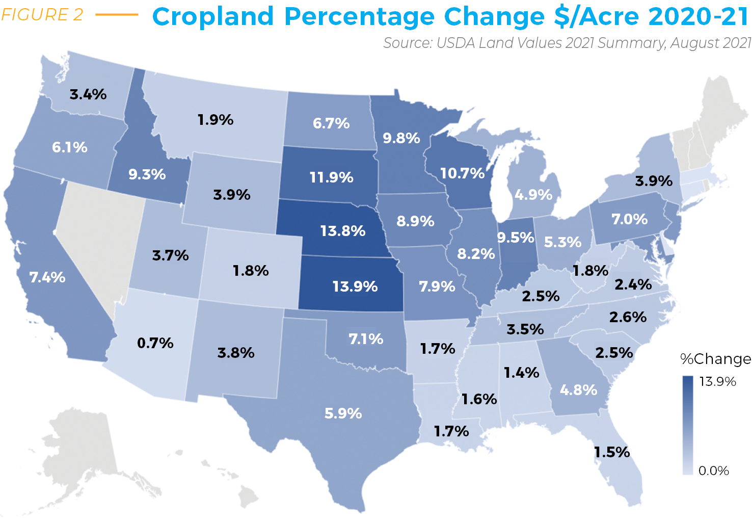
Figure 3 shows total return estimates based on USDA data by state derived from rental income plus appreciation less property taxes and maintenance expenses. In these cases, annual cash income can reliably be estimated on a consistent basis through time, and changes reported on a consistent basis. Importantly, these are estimates averaged across all properties in a state and thus mask the wide variation in individual experiences that could be expected to be encountered on a single farm. In any case, the performance is strong by historic standards, and even more impressive when compared to other investment opportunities such as equities or bonds.

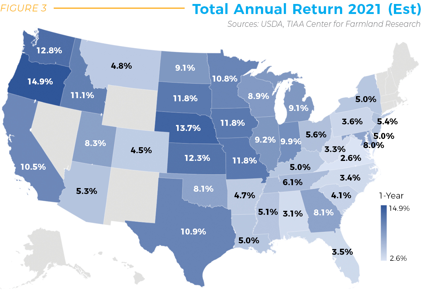
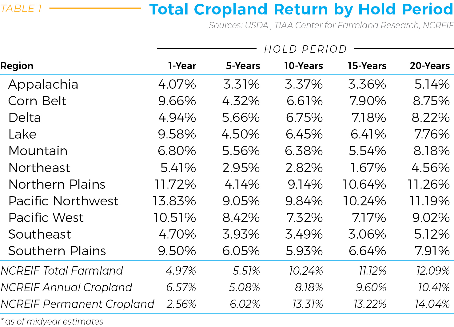
Table 1 provides additional historical context by aggregating this information into the same production regions used by the National Council of Real Estate Investment Fiduciaries (NCREIF) to group areas with similar production crops and practices and reporting total returns by hold period over selected intervals to 20 years. In addition to regional totals based on USDA data, the lower three rows provide total performance for assets held in the NCREIF index by type of production.

USING HISTORY TO LOOK FORWARD

It is important to consider the current economic and monetary system environment in which we are examining farmland, with particular attention to interest rates and expected growth rates for the economy. During the pandemic-induced shutdown, massive monetary stimulus was injected into the economy. Major disruptions took place in supply chains and labor markets, and considerable shifts occurred in consumer food consumption habits. During the subsequent upswing, there have been strong indications of price shocks in housing, transportation, food, and other sectors as well as debates about the permanence of the price increases and whether they are transitory effects from shortages and supply channel modifications or if there are signs of higher sustained inflationary pressures from misbalances in the monetary system. One key set of indicators to help demystify these issues is contained in the level of interest rates and broad-based measures of consumer price inflation. 

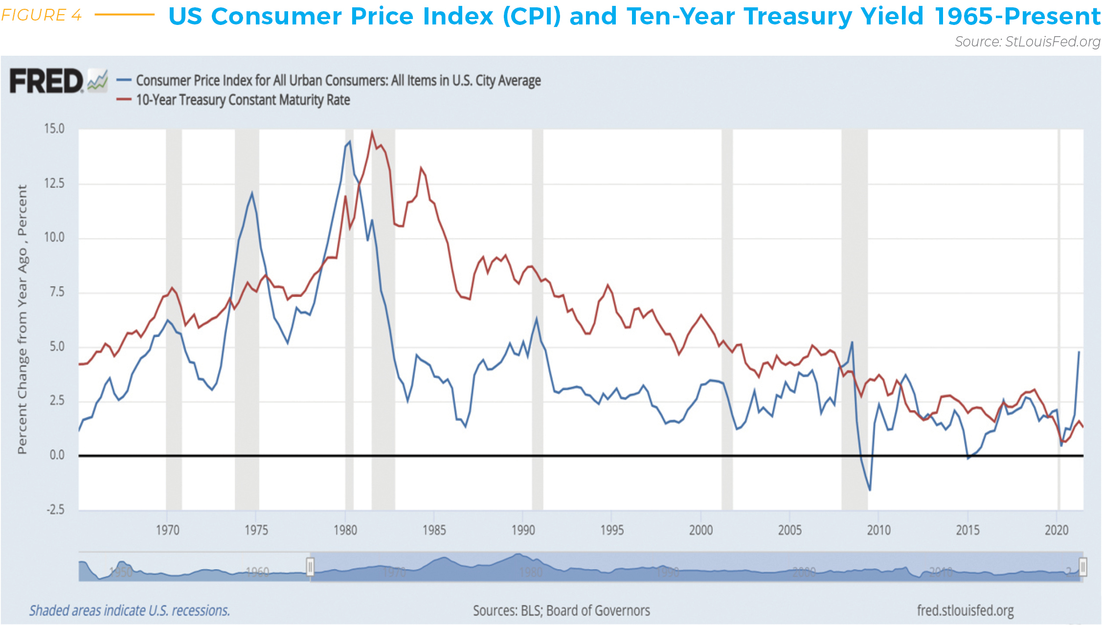
Figure 4 shows the Bureau of Labor Statistics (BLS) Consumer Price Index (CPI) along with the 10-year Treasury Constant Maturity (CMT-10) interest rate. Periods of recession are shaded in gray bars. A strong historic relationship exists between nominal interest rate movements and inflation with a simple correlation of about 67% from 1965 to present. The weakest statistical relationship took place in the 1980s. The CMT-10 is the most commonly used index of a risk-free capitalization rate reference around which relative credit spread and duration differences can be built to represent different asset cases and time periods.

What could be termed the Monetary Experiment of 2020-21 is currently being conducted with interest rates being held at low levels through direct intervention by the Federal Reserve (Fed). Continued assurances have been made that they can continue to manage growth rates through targeted interest rate and unemployment levels. Recent signals have begun to emerge that the Fed is acknowledging potential higher inflation, finding longer-term segments of the yield curve to be less responsive, and is beginning to target empirical inflation measures at higher levels than in recent history. 

Many would argue that we have entered a new longer-term regime of lower and more stable growth rates than occurred in the period from 1970 to 2000, so perhaps lower earnings may be in store for some time, and perhaps lower “normal” interest rates can be maintained as well.

In any case, it is a fair question to ask how farmland values would be impacted in the case of future interest rate increases and/or inflation shocks if these were to occur in the near future as that set of previous implied questions about future interest rates and inflation levels are resolved. 

To better gauge these effects, it is instructive to consider historic interactions and any changes in structural relationships that might affect that relationship going forward. Note that coming out of historical recessions, CPI levels often rise and sometimes “overshoot” during the restart of economic activity. Thus, the possibility of transitory inflation carries some historical precedent. Viewing the far right-hand side of the graphic, the rapid spike in the CPI and the relative stability of the interest rates raise questions about future inflation, and what we can learn about farmland’s response to similar shocks in the past. It should be noted that the causes of this recent recession and the components of the Personal Consumption Expenditures (PCE) and CPI measures contributing to price inflation have few historic analogs, and thus have few certain resolutions at this point.

Farmland is an immense asset class, but it is also one that has limited directly observable data on long-term returns at the level of the individual farm. In the items presented below, the asset class as a whole is considered through the use of a set of returns data at the state level and in various agricultural regions throughout the US from 1969 to present based on USDA data and maintained at the TIAA Center for Farmland Research at the University of Illinois. In simplest form, annual rates of returns are constructed as rental income plus appreciation less property taxes, divided by initial value. All series presented are converted to geometric annual returns for consistency. An aggregated index of the top 32 agricultural producing states is used as a proxy for the agricultural farmland market to compare to the CPI and Treasury yields. 

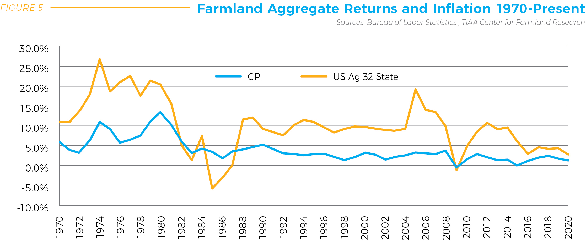
Some interesting features are evident in the graph over a long time period with differing monetary regimes and inflation rates. During the 1970s after the US went off the gold standard, inflation was largely unchecked. Inflation rates hit double digits, peaking at the start of the 1980s. These were also the halcyon days for agriculture, and farmers and lenders began promoting programs that later backfired under a perfect storm for agricultural producers. Multiple foreign crises then culminated in a grain embargo and oil market turmoil while fixed interest rates on farm mortgages peaked at nearly 18%. Inflation peaked at more than 10%, and farmland was caught in a credit-induced crisis. Thereafter, Treasury rates and inflation become more actively managed by the Fed with ensuing targets below 5% for the period that started in the late 1980s and persists through the present. 

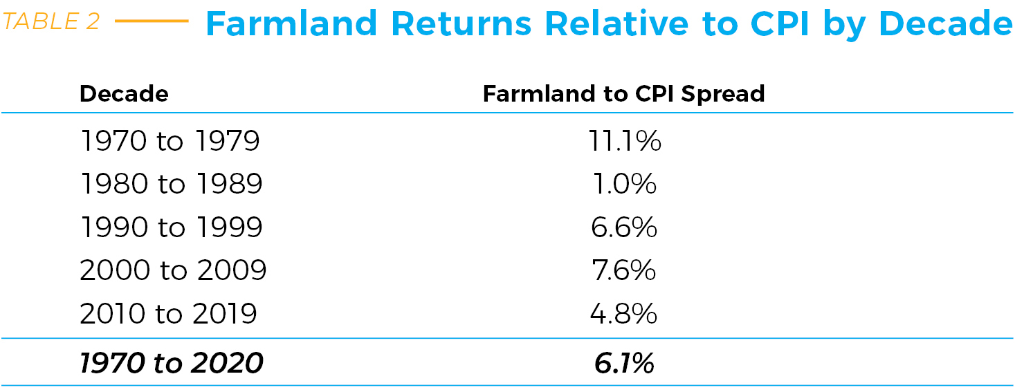
Table 2 summarizes the information in the graph in decade form. In the 1970s, the farmland price boom was the most important feature of returns. Annual appreciation routinely exceeded income. In the 1980s, farm income was positive, but the capital losses were greater than current income in both 1985 and 1986 with total returns of –5.8% and –3.1%, respectively. All other years in the 50-year period show total positive returns except 2009, which is considered to be a sympathetic response to broad market uncertainty generated by the housing crisis.

Individual state-level returns (not shown herein) have very similar patterns but display greater volatility. The majority of the variation in return in both cases is due to appreciation as annual rental income is a very smooth component of total returns on a relative basis.

Clearly, it is more difficult to buy farmland assets than to buy stocks or bonds. Although the transaction costs are higher, the hold periods and tax advantages associated with real assets help to even out initial disparities over time. Every parcel of farmland is unique, thanks to a host of factors including crop type, soils, and regional issues as well as external factors such as terminal locations for products. Increasingly, water rights, production practices, and environmental attributes impact local markets. 

Furthermore, farmland tends to be owned for longer periods of time and is often traded within families. This makes it complicated to assess large numbers of related parcels at any point in time. In fact, only 1.5% or so of regular row crop farmland changes hands annually at arm’s length. Thin market features do perhaps also offer supporting lower bounds to some regional markets. 

But, it is nearly always the case that farmland transactions are more complex and lack the uniformity of those in other asset classes. 

Fortunately, the farmland market is becoming more accessible and more understandable due to advances in ag-tech, improvements in informational sources, and the development of sophisticated and efficient financial channels as well — the financialization of the asset class appears to be in full swing.

This article was taken from the 2021 National Land Values Report. Click here to read the entire report.