
The Income Approach: What Earnings Tell Us About Land Value
This article is the first in a three-part series examining the primary methods used to appraise farmland in Iowa and across the Midwest.
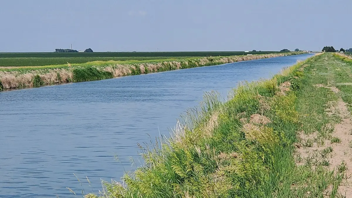
Originally published by Iowa State University. Co-authored by Rabail Chandio and Emily Oberbroeckling.
Iowa farmland serves as both a working asset and a long-term investment. While recent sales show what land sold for, the income approach helps explain why it sold for that amount by connecting value directly to the land’s ability to generate cash rent, crop profits, or long-term appreciation. In essence: What return can this land reasonably earn, and how does that compare to alternative investments? Rising interest rates, fluctuating grain prices, crop insurance guarantees, and investor demand all influence these expectations.
How The Income Approach Works
In economics, an asset’s value equals the present value of its expected future benefits. For farmland, those benefits come in the form of net operating income (NOI): income after property taxes, insurance, and management costs. When a buyer evaluates farmland, they are asking:
Expected income: What will cash rent or operating profits realistically be?
Risk: How stable are yields and prices?
Alternatives: How do expected returns compare to bonds, CDs, or other investments?
Just as a stock’s price reflects its expected future dividends, farmland’s value reflects the income it can reliably produce over time.
Two Ways To Apply The Income Approach
1. Direct Capitalization Method (the IRV (Income-Rate-Value) Approach)
The direct capitalization (cap) method is the most common technique used by appraisers, assessors, and agricultural lenders. It’s based on a simple relationship between income, rate of return, and value:
Value = Net Operating Income / Capitalization Rate i.e., V = I ÷ R.
This equation captures the essential link between income, value, and return expectations. It can be rearranged to highlight different perspectives:
I ÷ R = V; used to estimate value.
I ÷ V = R; used to find the implied rate of return.
R × V = I; used to determine the income a property must generate to justify its price.
To see how the income approach works in practice, consider a simple example. Suppose we want to know what return a buyer is earning on a recent sale. A farm brings in $250 per acre in net operating income and sells for $10,000 per acre. Using I ÷ V = R, we divide $250 by $10,000 to find a 2.5% cap rate, the return implied by the sale.
Now, imagine we want to determine the value of a farm based on its income and typical market returns. If a parcel generates $300 per acre in NOI and similar farms are trading at a 2.5% cap rate, we use I ÷ R = V. Dividing $300 by 0.025 gives a value of $12,000 per acre.
How To Interpret Cap Rates
Capitalization rates (cap rates) provide a quick snapshot of the relationship between farmland income and value, reflecting both market conditions and perceived risk. Low cap rates (around 2% or less) typically indicate strong demand, low interest rates, or high-quality land with stable income; in Iowa, top cropland often trades in the 1.5% to 3% range, while CRP tracts fall closer to 3% to 5%. Higher cap rates (5-6% or more) suggest greater risk or weaker demand. CRP acres or farms with livestock facilities, dwellings, or grain storage may generate more income, but their higher insurance, maintenance, and management costs, along with reduced flexibility, raise risk and push cap rates upward. Likewise, tracts with lower CSR2 soils, flood risk, or long-term program restrictions often trade at higher cap rates, even when gross rents appear strong, as limitations on use or resale narrow the buyer pool.
Several factors influence where capitalization rates settle in the farmland market.
Risk: Higher-risk properties typically have higher expense ratios, which reduces NOI and pushes cap rates upward.
Income stability: Predictable cash rent or program payments compress cap rates; volatile yields or uncertain tenants expand them.
Interest rates: Higher borrowing costs increase investor-required returns, which in turn raise capitalization rates and lower property values.
Local market demand: Limited supply and strong buyer competition often compress cap rates, raising land values.
2. Discounted Cash Flow (DCF) Model
The capitalization rate used in the direct capitalization method can be viewed as a simplified version of the discount rate used in a Discounted Cash Flow (DCF) model, applied when income is expected to remain constant indefinitely. Direct capitalization assumes (1) annual income remains the same each year and (2) that income continues forever.
In contrast, the DCF model offers far greater flexibility, making it particularly useful for long-term investment analysis or situations where rents, yields, or resale values are likely to fluctuate over time. Instead of capitalizing a single year’s income, the DCF approach projects net income for each future year and then discounts those cash flows back to their present value. This makes the method especially helpful in markets where rents may rise, crop returns may vary, or expected resale value is an important component of the investment.
In this framework, the discount rate (sometimes referred to as the yield rate or internal rate of return (IRR)) represents the return required by investors based on the property’s risk profile. The difference between these terms lies in how they are used:
The discount rate is applied prospectively to determine value: Given a required return of 7%, what is this property worth today?
The IRR is calculated retrospectively: Given this purchase price and these cash flows, what return am I earning?
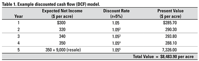
To see how the DCF model works, consider a parcel expected to generate rising net income over five years, followed by resale (Table 1). Each year’s income is discounted back to present value using a 5% discount rate. For example, $300 of income in Year 1 is worth about $285.70 today ($300 ÷ 1.05), and $350 of income plus a $9,000 sale in Year 5 is worth roughly $7,326 ($9,350 ÷ 1.055) in present-value terms. Summing the discounted values for all five years produces a total present value of approximately $8,484 per acre. Under these assumptions, the land would be worth about $8,500 per acre if investors anticipate moderate rent growth and an eventual resale price of $9,000 per acre.
Strengths and Limitations
The income approach remains one of the most useful tools for interpreting farmland values because it directly connects price to earning power, risk, and long-term economic expectations. Its strength lies in its clear logic: when rents, expenses, interest rates, and risk change, the model shows exactly how those changes are reflected in land value. It is especially effective for evaluating cropland with stable rental income and limited improvements.
However, it also has limitations. The approach is sensitive to small adjustments in discount rates or rental assumptions, and its accuracy depends on reliable, localized data. It may also overlook non-economic motivations such as sentimental value, strategic expansion, or tax considerations that play a role in many farmland transactions. Even so, the income approach provides a disciplined economic lens for interpreting how broader forces (such as rising interest rates, crop insurance structures, commodity price expectations, inflation, or policy shifts) translate into market values. When paired with comparable sales and cost approaches, it offers a well-rounded view of the farmland market and the drivers shaping land values across Iowa and the Midwest.
Agriculture
Crop Insurance
Energy Management
Industry Insights
Land Auctions
Land Investment Expo
Land Management
Land Values
News & Events
Real Estate

Peoples Company proactively works to anticipate the needs of those in the agricultural sector. Our monthly email publication keeps readers in the know about everything land.
